 |
|
This page provides the following material concerning shadow:
Notes: Adjacencies between shared edges should be declared explicitly. Correct surface normal orientation, pointing into a model's interior, is not necessary for this application expect in face partitioning.
Input objects may be surfaces, shells, instances or groups. All are converted to shells internally.
Visibility analysis provides those regions visible (or hidden) from a given viewpoint. Fulcrum point accessibility analysis determines region accessible (or inaccessible) by a semi-infinite probe (extending to infinity in one direction) whose axis is constrained to pass through the given fulcrum point. The probe itself need not pass through the fulcrum point, only it's axis; allowing for access both towards and through the fulcrum point.
In addition to visibility and accessibility partitioning, model back/frontface partitioning and contour extraction and classification can be performed. These operations are typically quicker and more robust then visibility and accessibility partitioning.
The type of partitioned regions to be kept can be specified as those satisfying the desired analysis (eg visible), not satisfying the desired analysis (eg hidden), or split (eg both visible and hidden). Those regions satisfying the analysis are colored white, while those that do not are colored blue.
Contour classification depends on the type of analysis chosen. Face partitioning extracts contours but performs no classification. Contours extracted with either visibility or accessibility analysis are segmented at all junctures (T, cusp, or merge) in a contours image projection. With visibility analysis, contour segments are assigned classes based on the visibility of each segment. With accessibility analysis, contour segments are assigned classes based on the accessibility of each segment. Each segment is assigned a color based on it's class. Contours can be extrated in any of three spaces: paramateric model space, Euclidean threespace, or projected image space. All model contours including interior surface contours, model boundary contours, shared edge contours, and surface discontinuity contours are extracted.
Partitioned regions (or extracted contours) are written to stdout.
shadow wavy.a1 > wavy.vis.a1
aset shadow.keep not
shadow wavy.a1 > wavy.vnot.a1
aset shadow.keep split
shadow wavy.a1 > wavy.vsplit.a1
 |
 |
 |
The three output files are illustrated respectively above. The first two are illustrated as seen from the specified viewpoint. The split partitioning is illustrated from a different vantage point then that used for the analysis.
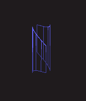
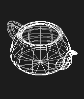
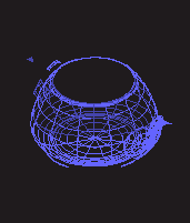
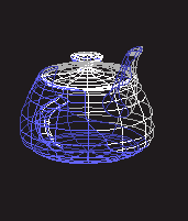
aset shadow.analysis access
shadow teapot.a1 > teapot.ais.a1
aset shadow.keep not
shadow teapot.a1 > teapot.anot.a1
aset shadow.keep split
shadow teapot.a1 > teapot.asplit.a1
 |
 |
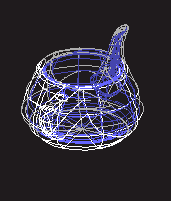 |
The three output files are illustrated respectively above. The first two are illustrated as seen from the specified fulcrum point. The split partitioning is illustrated from a different vantage point then that used for the analysis.
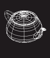
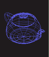
aset shadow.analysis front
shadow teapotl.a1 > teapotl.fis.a1
aset shadow.keep not
shadow teapotl.a1 > teapotl.fnot.a1
aset shadow.keep split
shadow teapotl.a1 > teapotl.fsplit.a1
 |
 |
 |
The three output files are illustrated respectively above. The first two are illustrated as seen from the specified viewpoint. The split partitioning is illustrated from a different vantage point then that used for the analysis.
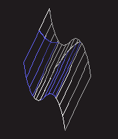
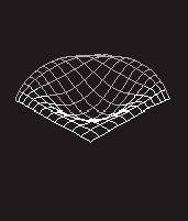
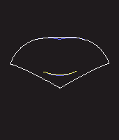
aset shadow.view_pt 100,80,100
aset shadow.cntrs_only on
shadow dimple.a1 > dimple.cvisib.a1
aset shadow.analysis access
shadow dimple.a1 > dimple.caccess.a1
 |
 |
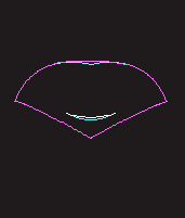 |
The first image illustrates the dimple surface. The projective image mappings of the contours are illustrated respectively in the remaining two as classified for each analysis type.
 Alpha_1 User's Manual Version 98.01.