 Alpha_1 User's Manual
 Alpha_1 User's Manual
The combineShells operation in c_shape_edit modeler uses the same underlying surface-surface intersection library code, but is inline in a modeling session where you have to wait for it. This is okay on small-to-medium sized models, but hand, set_op has the advantage that it can be invoked in the background, on another workstation or server, with huge models.
Table of contents for this page:
- Set Operations Overview
- Modelling with set operations and sculptured surfaces.
- Preparing a Model for Booleans
- Names, Adjacencies, Shells, and Orientation Issues.
- Running Set_op
- Commands for setting flags and running the set_op program.
- Summary of Hints
- A checklist of common problems.
The "combiner" implements the "boolean set operations" which are the basic operations of the Constructive Solid Geometry (CSG) modelers. These operations were originally developed to allow modeling of a large class of objects from combinations of regular solid primitives. The extension of these boolean operations to sculptured surface primitives allows the designer more freedom in creating part models, but introduces complexity and subtlety to both the implementation and use of these operations.
The domain of discussion is broader when we discuss boolean operations in the context of a surface based modeler. The familiar operations of union, intersection and difference are intuitive and easily explained in terms of cubes and cylinders (solid objects) but are not as straightforward when applied to surfaces which are not "closed" and therefore do not trichotomize space into "inside", "outside" and "on" the part.
Therefore, we describe in more detail the shell object which was introduced earlier. A shell represents a grouping of surfaces which may be connected ("sewn together") along their appropriate edges by adjacency declarations. The boolean operations are stated in terms of these shells. The results of the boolean operations are represented by an approximation of the true intersection curves between these shells and regions of the surfaces bounded by these intersection curves. The results are represented as trimmed surfaces, contained in shells.
The rest of this section provides an overview of the procedure for performing boolean operations.
One first describes the geometry of the surfaces which will represent the part to be modeled. This is covered under Surface Constructors, and it is assumed for this discussion that only a collection of surfaces has been constructed (no procedures which generate shells have been used). Further, the surfaces have an inside and an outside, that is, the orientation of the surface normal is used to denote which side of the surface is the solid. Recall that the normals point "into the part".
Second, construction of a shell from surfaces is done by:
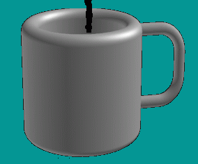
This choice of example, using very simple geometry, i.e., a surface of revolution for the body, round planar surfaces for the floor and base and a simple tubular handle is meant to show a variety of ways in which surfaces are combined to make a solid. Specifically, the body will be attached to the floor and base using declared adjacencies, the handle surface will be closed into a tube by using a self-referential adjacency declaration and the handle surface will be attached to the body using a boolean operation.
As one refined the design of the cup so that, for instance, the base of the cup became a more ornate pedestal or Grecian column, it might be more desirable to attach it to the body using a boolean operation. The strategy used to model an object may be easily changed as the design progresses. The point of this example is to illustrate different ways to join surfaces into solids.
The objects on which the boolean operations are performed are a higher level construct than surfaces for several reasons. These objects are called shells and they are composed in several ways. Historically, it has been common practice to model objects as collections of bounded parametric surfaces which meet at their boundaries. For example, a cylinder or a box can be modeled exactly, without need for any trimming or boolean operations by creating bounded surfaces which represent the "faces" of the object. This type of modeling provides a very concise means of representing shapes. In order to extend the utility of these surface models to the domain of solids which can then be combined using boolean operations, the connectivity of these surfaces must be made explicit so that the algorithm which evaluates the combination expression does not have to deduce information which is already known at an earlier stage in model construction. This information is used to connect intersection curve pieces which are later used to classify the surface segments of the resulting combined object.
This technique of defining surfaces which enclose a solid and declaring their connectivity can be used to encapsulate the definition of objects of interest which contain sculptured surfaces and thus are much more general than the simple primitives of CSG based geometric modelers.
It is also common in modeling to think of a geometric feature as a set of surfaces which are not contiguous, but which logically define a feature of the model, for example, if the cup design were extended to provide two handles, one still might think of the "pair of handles" as the handle when describing the whole cup as "body+handle".
In summary, a shell can represent
Body: shell( Cup, Roof, Floor );
Associated with the topologically rectangular surface is a control mesh which (partially) defines the shape of the surface. It is represented by a matrix of points. The boundary of the surface which is associated with the first row of the matrix is called the "top" boundary of the surface. The boundary of the surface which is associated with the first column of the matrix is called the "left" boundary. The "bottom" and "right" boundaries are the obvious mates. (Incidently, as you look at the matrix in this way, the surface normal of the surface points into the solid which it represents. The normal is determined with a right-handed cross product UxV at the top left corner.) The getBoundary routine is often useful for determining the location of a desired boundary, by highlighting the resulting curve on the display.
Given surface names and boundary identifiers, adjacencies are declared by the designer by indicating which boundaries are coincident.
Adjacencies are declared with one of the three adjacency constructors: mkAdjacentFull, mkAdjacentPartial, or mkAdjacentTrim (see the chapter [Leaving Shape_edit]). There are two forms of adjacencies, intersurface and intrasurface.
If one surface was used to form a tubular handle for the cup, one could close the seam in the handle by the the following declaration:
mkAdjacentFull( HandleSrf, 'Left, HandleSrf, 'Right );
If one used a surface of revolution to form the inside and outside of
the cup and several discs to make the inside floor and outside bottom
of the cup, the body of the cup could be "sewn" together in the
following style:
     % Declare the attachment between the floor and the
     % body of the cup.
     mkAdjacentPartial( Body,  'Bottom, 0.0, 1.0,
                        Floor, 'Right,  nil, nil );
     mkAdjacentPartial( Body,  'Bottom, 2.0, 3.0,
                        Floor, 'Left,   nil, nil );
     mkAdjacentPartial( Body,  'Bottom, 1.0, 2.0,
                        Floor, 'Bottom, nil, nil );
     mkAdjacentPartial( Body,  'Bottom, 3.0, 4.0,
                        Floor, 'Top,    nil, nil );
     ...
Fortunately, the code which generates surfaces of revolution does
this automatically when endcaps are requested, so the designer
doesn't have to.
dumpA1File( list( Body, Handle ), "coffeecup.a1" );
set_op filesTo specify the operations to be performed, we use the aset command. Set union is given as a "+", set intersection as a "*", and set difference as a "-". The cut operation is given as "/". If the input file contains a number of shells which are to be operated on in sequence, they may all be done in a single invocation of the set_op program by specifying a sequence of operations as illustrated below. (One caution: the asterisk is a special character for the C-shell, so you will want to enclose sequences containing intersections in double quotes.) Set intersection is the default operation if nothing is specified.
- Output
- binarystream Trimmed surface data, contained in shells, representing the boolean result.
- files
- filelist Files to be used in the boolean combination.
     aset set_op.operations +
     aset set_op.operations --
     aset set_op.operations "*---"
In the last example, if the input file contained five shells, the
intersection of the first two would be computed first, then each of the
succeeding three shells would be subtracted from the result of the
preceding operations. For our example, the command for actually computing the boolean operations is:
     aset set_op.operations +
     set_op coffeecup.a1 > cup.trims.a1
An alternative form, which allows arbitrary ordering of the
operations on the shells is to use a fully parenthesized
specification, referring to the shells by single letter names which
are assigned based on their order in the file. So, the first shell
in the file is "a", the second one is "b" and so on. The same
operation symbols are used: "*", "+", "-", and "/". In
addition, a negation operator, "~", is also available, but must
always be enclosed in parentheses. So you could use:
     aset set_op.operations "( b - a )"
     aset set_op.operations "( ~a )"
The following additional options for the set_op program can be set
using the a1defaults mechanism .
Default values are given in parentheses.
The set_op program now (optionally) uses a new algorithm based on numerical techniques to find the "true" intersection of the edge curves of one surface versus the other surface. A planar bilinear approximation is used only to provide initial parametric values for the numerical iteration. Optionally, intersection curves can be filled in between the points where an edge curve pierces the other surface to form a smoother curve.
- set_op.operations
- (*) As described above, this specifies the sequence of operations which will be performed on the sequence of shells in the input file.
- set_op.obj_resolution
- (0.01) Set the tolerance at which the boolean operations will be computed. This number says that the faceted approximations of the surfaces which are being intersected will be within this distance of the true surface. Note that this does not necessarily imply that the computed intersection is within the same tolerance of the true intersection. The default value of 0.05 is usually too large for models with coordinates in the range of small integers (up to 10, say). More typical values used are in the range 0.02 to 0.005.
- set_op.curves_only
- (off) This is useful for trying to figure out what went wrong if there is an error generated by set_op. The intersection curves of the first boolean operation in the sequence are output, and can be examined with other utility programs (e.g., viewa1, tk3d).
- set_op.increase_density
- (off) Attempt to improve the accuracty of the computed intersection curves by using an iterative numerical scheme to add new intersection points between those computed by the intersections of the faceted surface approximations.
- set_op.max_iterations
- (8) The maximum number of iterations which will be applied in trying to improve the accuracy of any particular control point. (Of course, the result usually converges before this many iterations are necessary.)
- set_op.same_point_tolerance
- (1.0e-6) Set the tolerance for curve improvement. The improvement is declared to converge when two successive iterations yield a solution that is within this tolerance.
- set_op.join_tolerance
- (1.0e-5) Set the tolerance for joining curves across surface boundaries. Points which are closer than this are treated as identical and may be joined.
- set_op.force_curve_tolerance
- (.02) Set the tolerance used for forcing intersection curves to meet along a shared edge. If two intersection curves intersect a shared edge within this tolerance in parametric space, the two curves will be forced to intersect at the same point on the shared edge.
- set_op.stages_debug
- (0) Print status information at each stage of the set operation. Useful for determining which operation out of several has failed. A value of 1 results in brief messages after each stage in the set operation to be printed while a value greater than 1 causes information about the output trimmed surfaces to be printed as well.
The following default values control the new algorithm:
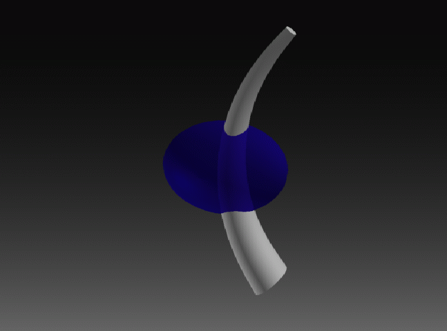
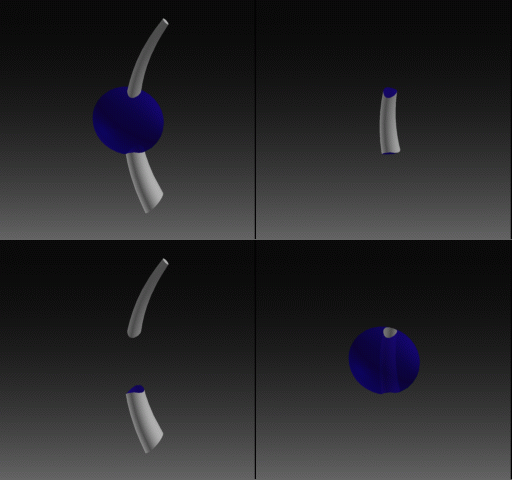
One useful aid when problems are encountered is the set_op.dump_leaves flag, which is a variant on set_op.curves_only. If this is turned on, the subdivided "flats" from the two shells will show up in blue and red, and the intersection curves will be white. This can be useful in finding out why an error occurs in the output phase, for example if intersection curves don't meet to form valid trimming loops.
- set_op.triangular_approx
- (on) The (old) triangular approximation is the default. To use the new algorithm, turn off this flag.
- set_op.normal_spread_angle
- (30) Used to control the amount of subdivision performed, it is the maximum angular spread in degrees of the normal surface direction vectors such that a surface will be considered "flat".
- set_op.same_point_tolerance
- (1.0e-6) Used to determine whether two points are considered the same or not: if the distance separating the points is less than the indicated value, they are considered the same. If this tolerance value is decreased, more iterations are required for the numerical algorithms to converge.
- set_op.increase_density
- (off) Used to turn on the curve marching between intersection points. It will produce smoother intersection curves.
- set_op.step_size
- (0.02) Used to control the distance in E3 between intersection points when set_op.increase_density is on.
- set_op.dump_leaves
- (off) Used for debugging problems which occur. Dumps geometry which can be viewed to localize problem areas.
The bottom line is that the new algorithm should produce very accurate intersection curves without using huge amounts of memory, which occurs when using very small resolutions with the triangular method. It also provides the necessary framework for solving the surface coincidence problem. One disadvantage is that there is nothing comparable to using a crude resolution with the triangular method, the closest one can get to that is to have increase_density off and use larger values for set_op.same_point_tolerance and set_op.step_size. When compared to using a very fine resolution with the triangles, it takes a similar amount of cpu time, but much less memory.
 Alpha_1 User's Manual Home Page