Alpha1 User's Manual

Alpha_1 Tutorial

This tutorial is designed to give a new user of Alpha_1 an overview of how one normally interacts with the system. Enough information is given so that the reader can try out the operations described, but the explanations are limited so that the overall direction is not lost in the detail. To get a full idea of what operations are available it is necessary to read the individual application manuals or skim over the supplementary summarizes of routines.

After this tutorial, a user should be able to interact with the command language interface to c_shape_edit from within emacs, create simple models and display them either as line drawings or shaded raster images, use simple boolean set operations, and save the results of their work for use at a later time.

The tutorial includes small number of sample constructions exhibiting a range of applications from stylized modeling for graphics (a wine goblet) to real mechanical parts which are to be manufactured (a simple bracket).

Preliminaries

This tutorial assumes that you have at least a minimal knowledge of Unix, the X Window System, and emacs. If you don't know how to log in, start X, find some files, and edit them, it will probably be difficult to follow. The tutorial also assumes that you have an installed Alpha_1 system on which to try these examples and are setup to do so. To get a quick overview and introduction to the system, see the Alpha_1 Introduction. To get setup to use Alpha_1 and try the examples in this tutorial, see Getting Started with Unix. Illustrations are provided throughout the tutorial, but is useful to try the examples as you read as well. Hint: use the X Window System cut and paste facilities to avoid typing in all the examples.

Now log in, start up X (if necessary) and emacs, and find any file which ends in a ".scl" suffix, such as test.scl. When you load the file, the emacs mode line should say "(Scl)", indicating that emacs has recognized that you have read an SCL file and will be running c_shape_edit under emacs.

Now type (in the "test.scl" buffer):

2 + 2;

At this point you are just entering text in a buffer, and emacs treats it like any other buffer. To indicate that you want the command executed by c_shape_edit, position your cursor anywhere on the line you just typed and type "Meta-e" (or escape-e, or Alt-e). This should result in the message "Starting c_shape_edit..." appearing in the emacs mini-buffer. Emacs will then split your display into two windows (if there is only one current window), and start up c_shape_edit as a sub-process. One window will contain your input buffer, "test.scl", and the other will be the output buffer, where all the (text) output from c_shape_edit is displayed. Your emacs window should now look something like this:

Although it is possible to type commands in the output window, things are generally much less confusing if you type all your commands in the input buffer.

When c_shape_edit is first started, you see the message banner and c_shape_edit prompt in the output buffer. Since you have already requested that a command be executed, emacs goes ahead and sends the 2 + 2; line, c_shape_edit executes it and prints the result, and gives you a new prompt indicating that it is ready for your next command.

Your cursor will be positioned on the next line in your input buffer, ready for you to type another command. You can continue typing commands, using M-e to execute them whenever you like. Remember that you must use "M-e" to get the line executed -- using "return" just puts a new (blank) line in the buffer, but doesn't execute the previous line. Also note that the semicolon is crucial. It denotes the end of the statement, and c_shape_edit won't try to evaluate what you have said unless it finds a semicolon. In fact, it will continue to read lines out of your buffer until it finds a semicolon or runs out of input.

You can exit c_shape_edit by entering the command quit;. If you try to exit your emacs while c_shape_edit is still running, emacs will ask you to confirm whether you want to kill the sub-processes before you exit.

Comments in c_shape_edit are denoted by the "pound" character #. Comments are entirely optional, but will be used throughout the rest of this tutorial to explain c_shape_edit commands.

Now try to create some simple geometry in c_shape_edit:

P1 : pt( 0, 0 );       # Create a point, and call it P1.
P2 : pt( .7, .7 );
LineA : lineHorizontal( 0.5 );  # Horizontal line at y = 0.5.
LineB : lineThru2Pts( P1, P2 ); # Line through P1 and P2.

Your emacs window now looks something like this:

Basic SCL Terminology

You will notice that the typical SCL command looks something like this:

 ObjectName : constructorName( Arg1, Arg2, ... );

This command creates or modifies the object named ObjectName. The constructor (or constructor function) used to do so is named constructorName. The arguments to the constructor are the comma-separated list of object names Arg1, Arg2 and so on. Numbers and basic arithmetic expressions can be used as arguments as well as object names. They can also be assigned names like any other object. Here is an equivalent model for P2 and LineA above:

PtCoord : .7;	# Named numeric parameter.
P2 : pt( PtCoord, PtCoord );
# Simple expression used as an argument.
LineA : lineHorizontal( PtCoord - 0.2 );

Note on Names

All constructor names, names for objects that you create, and names of built-in objects are insensitive to upper or lower case. That means Origin and origin are the same name. By convention, names of objects begin with an uppercase letter and names of constructors begin with a lower case letter. Multi-word names, like lineHorizontal use uppercase letters to separate the words.

Displaying Geometry

As soon as you begin constructing geometric objects, you will want to see them on the graphics screen instead of looking at the text output of c_shape_edit. You must start up a companion process (program) to communicate with c_shape_edit to manage the graphics. To do this, start the motif3d program by typing motif3d& to your Unix shell (not the emacs window!).

Viewing Controls in Motif3d

The motif3d window consists of a menu bar on the top, a panel of viewing controls on the right, and a drawing area for 3D display. Here is the basic layout:

Interactive view modification is accomplished by clicking and dragging with the middle mouse button in the drawing area (the black area in the above image) of the motif3d window. The top section of "radio buttons" on the viewing control panel is used to select which viewing transformaton is performed. Here is a fullsize view of the control panel.

Some viewing tranformations, like Scale associate left and right mouse motions with the transformation (right for larger, left for smaller in this case). Others, like XY Pan, associate all mouse movement (up, down, left, and right) with the transformation. The rest of the buttons on the viewing panel select predefined views or change other aspects of the viewing and are fairly straightforward. See the Motif3d/Viewa1 Manual for more information.

Viewing Commands in C_Shape_Edit

In order to get objects displayed once a motif3d window is active, we need to "show" them. This can be done with the c_shape_edit show command. Try the following command (entering it into your "test.scl" buffer, and executing "M-e" as before):

show( P1, P2, LineB );     # We created these earlier.

The motif3d window should now look something like this image.

There are five basic viewing commands in SCL, show, unshow, highlight, unhighlight, and select. Each takes a comma-separated list of names as the arguments as shown above. (Advanced emacs users can find out about emacs bindings for these commands by using C-h m in your "test.scl" buffer.)

Now that something is shown in the motif3d window, try selecting XY Pan mode and change the view as described above.

In the next section, we will begin an example of the construction of a model of a wine goblet. To prepare for that clear the motif3d window by selecting Clear from the View menu.

Wine Goblet

The modeling example we use in this section is the wine goblet in this ray-traced image:

The SCL commands for this model are in the file:

$A1ROOT/man/html/tutorial/examples/goblet.scl

You can read this file into your emacs and try the commands as you read through the following sections.

The wine goblet model is a "swept" surface constructed from four curves. The axis curve is the path of the sweep. The cross-sections (a square and a circle) are the curves that are swept along the path. Finally, the profile curve determines how the cross-sections are scaled as they are swept along.

Profile Curve Construction

First we will construct the profile curve which defines the basic shape of the goblet (its "profile" when viewed from the front). To do so, we define a set of control points that roughly describe the shape

# Control points for a goblet shaped profile curve.
<<
    GobPt1 : pt( 0.0,  0.24 );
    GobPt2 : pt( 0.05, 0.24 );
    GobPt3 : pt( 0.1,  0.24 );
    GobPt4 : pt( 0.15, 0.04 );
    GobPt5 : pt( 0.2,  0.04 );
    GobPt6 : pt( 0.25, 0.04 );
    GobPt7 : pt( 0.30, 0.16 );
    GobPt8 : pt( 0.35, 0.16 );
    GobPt9 : pt( 0.39, 0.04 );
    GobPt10 : pt( 0.6,  0.04 );
    GobPt11 : pt( 0.6,  0.32 );
    GobPt12 : pt( 1.0,  0.24 );
>>

This first thing to notice is the use of braces << ... >> to group a set of SCL commands into one command. In emacs, put your cursor on the line with the << and execute "M-e". All the commands up to the >> are executed. Now show the points in motif3d and adjust the viewing so you can see them all.

show( GobPt1, GobPt2, GobPt3, GobPt4, GobPt5, GobPt6,
      GobPt7, GobPt8, GobPt9, GobPt10, GobPt11, GobPt12 );

Now we will use a simple B-spline constructor to make a smooth curve from the control points:

# Note that the profile curve represents a function of X.
GobletProfile : uniOpCrv( cubic, 
    array( GobPt1, GobPt2, GobPt3, GobPt4, GobPt5, GobPt6,
	   GobPt7, GobPt8, GobPt9, GobPt10, GobPt11, GobPt12 ));
show( GobletProfile );

Your motif3d window now should look something like this:

This construction introduces two new constructors and the concept of nested constructors. The array constructor is a general constructor for a group of objects (of arbitrary number). Other constructors (such as uniOpCrv) often require an array as one of their arguments. The result of the array constructor could be assigned a name like any other constructor and that name could be referenced throughout the model. In this case, the array is only used in one place, so the constructor is nested as one of the arguments to another constructor.

The uniOpCrv constructor is the simplest B-spline curve constructor. The first argument is the order of the curve, which is the polynomial degree of the desired curve plus one (see the Spline Introduction for the basic terminology for B-splines). In this case we get a cubic curve. The second argument is an array of points which are called the control points and roughly define the desired shape. The order is the minimum number of control points necessary. This constructor is meant to hide some details of the B-spline curve by using a uniform knot vector and Open end conditions (hence the name) as defaults.

Axis Curve Construction

The axis curve for the sweep is constructed as follows:

# Use a linear axis curve. We degree raise the axis to a cubic
# to get a resulting sweep surface that is smooth.
GobletAxis : raiseCrvOrder( profile( pt( 0, 0 ), pt( 1, 0 )),
			    cubic );

This nested construction first uses the profile constructor to make a simple linear curve between two points. Because we are going to eventually use the axis in a sweep, we use the raiseCrvOrder constructor to make a cubic curve out of the linear one.

Cross-Section Curve Contruction

It is not necessary to construct a circular cross-section for the sweep because we can use a built-in object named UnitCircle (radius of 1). We construct the square cross-section using the profile constructor:

UnitSqrSec : profile( pt(1,1), pt(-1,1), pt(-1,-1),
		      pt(1,-1), pt(1,1) );
RotUnitSqrSec : objTransform( UnitSqrSec, rz( -45 ) );

The profile constructor takes an abitrary number of arguments and "connects the dots" to make a curve. Above it was used with two points, here we use five points, repeating the first one, to make a square. In order for the start of the square to line up with the start of UnitCircle we must rotate the square by -45 degrees (around the Z axis) using the objTransform operation.

Now we must specify how the cross-sections are to be used with respect to the axis curve. The axis curve is parameterized from 0 to 1. This means that a number between 0 and 1 is associatied with a point on the curve a percentage of the distance between the beginning (0) and the end (1). We need to create two arrays to use the sweep constructor: an array of cross-section curves, and an array of parameter values:

SectionCrvs : array( RotUnitSqrSec, UnitCircle );
SectionParams : array( 0.1, 0.15 );

These two arrays will be used to specify that as we sweep along the axis curve the square cross section should be used from parameter value 0 to 0.1. From 0.1 to 0.15 a blend of the square and circle cross sections will be used and from 0.15 to the end of the curve the circular cross section will be used.

The Sweep Construction

Now all that is left is to make the sweep surface itself. To do so, we will use the generalSweep constructor:

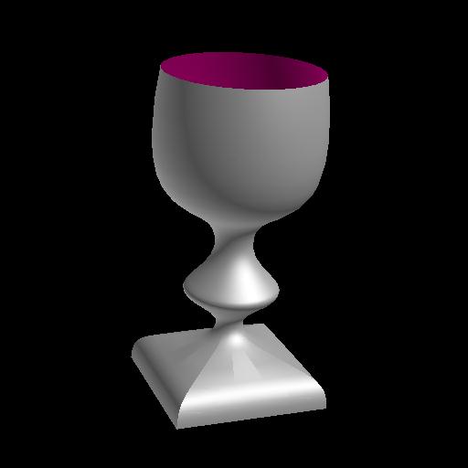
Goblet : generalSweep( GobletAxis, SectionCrvs, SectionParams, 
		       "arc_length_blend", GobletProfile, false );

The first five arguments are the axis curve, the array of cross-sections, the array of cross-section parameter values, the type of blending to use, and the profile curve. The surface should look something like this in your motif3d window:

Constructor Options

The last argument used above for the generalSweep constructor is an optional specification for orientation of the cross-sections. We have used the keyword false to indicate the default orientation is desired. The names true and false are keywords in SCL (and are case sensitive) and are often used to specify options for constructors.

Another method for constructor options is to use charater strings, such as "arc_length_blend" above. For a particular constructor there is usually a small set of valid option strings for a particular argument. In this case, the generalSweep constuctor has a number of options for blending cross-section curves.

Making a Rendered Picture

We will consider our goblet model complete at this point, even though it actually needs a little more work to make a true model that encloses some space. What we have designed so far is just a surface: it has no thickness. However, we want to cover some other aspects of Alpha_1 in the remainder of this tutorial.

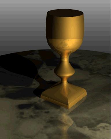
One of the most important utilities you will need to know how to use is the render program for producing shaded raster images of your models. Smoothly shaded color pictures can often give much more information about the shape of an object than line drawings can.

Saving Data Files from C_Shape_Edit

In order to run the rendering program, we must first save our model data to a file from c_shape_edit. We use the c_shape_edit command dumpA1File to create a binary Alpha_1 data file:

dumpA1File( array( Goblet ), "/tmp/goblet.a1" );

Since dumpA1File is not a contructor (it does not create an object) there is no object : on the lefthand side. This is called a side-effect function. The arguments are an array of objects to be saved, and a Unix file name given as a character string. By convention, we always use the ".a1" file extension to identify binary Alpha_1 data files.

Choosing a Viewpoint

Now you are ready to leave c_shape_edit and get ready to run the render program from the Unix shell. The first thing to know is that the objects to be rendered and the viewpoint from which to render them are specified separately. The dumpA1file command used above only saved the geometric surface information. Unless a front view with default scaling is desired (hardly ever the case) the viewpoint information must be explicitly provided (with another ".a1" file).

We can use motif3d to save viewpoint information in a binary Alpha_1 (.a1) file. First, position the goblet surface in motif3d in the orientation you wish to produce a rendered image. Next, choose Save View Matrix As... from the File menu. Now you should see a dialog box like this:

Type the file name /tmp/mat.a1 (as shown) in the dialog box and click the OK button. This writes the current viewpoint (i.e.: view matrix) into the .a1 file.

In addition to doing this with motif3d, the viewa1 program is available. This program is virtually identical to motif3d except that it reads .a1 data files as input as opposed to communicating interactively with c_shape_edit for input. This is convenient if you wish to select and store viewing information or just look at an existing .a1 file without running c_shape_edit and motif3d together. Run the program from the Unix shell on your .a1 data file by just providing the name of the file:

viewa1 /tmp/goblet.a1

Once viewa1 is running, you can use save a view matrix exactly the same as described above for motif3d.

Running Render

Now you are ready to run the rendering program. We use the ".rle.Z" extension to denote image files created by render because they are stored in the Utah Raster Toolkit (URT) run-length encoded format (.rle), and because they are automatically compressed to save disk space (.Z). Start the rendering process by giving render the input files and redirecting the standard output to a ".rle.Z" file. Since render usually takes a little while, the ampersand on the end of the line is often a good idea.

render /tmp/mat.a1 /tmp/goblet.a1 > /tmp/goblet.rle.Z &

The getx11 program (part of URT) or the commonly available xv program can be used to view the image. The getx11 program handles compressed files, so you can use it to check on the progress of render. The xv program does not handle compressed files, but you can uncompress the .rle.Z file when render is finished and then us xv as a viewer. The results of the example above should look something like this:

Advanced Rendering

More realistic images can be produced using the ray program which renders images using a ray-tracing method. We will show a simple example illustrating the most useful properties.

The modeling example we use in this section is a flat surface and a ball (sphere) shown in this ray-traced image:

The SCL commands for this model are in the file:


$A1ROOT/man/html/tutorial/examples/rendering.scl

Model

The model in this example is extremely simple:

Srf : flatSrf( linear, linear, 2, 2 );
Ball : sphere( pt( 0, 0, .25 ), .25 );

The first command makes a flat surface from coordinates (-1,-1) to (1,1). The second makes a sphere that touchs the flat surface at a point.

Attributes

Now we set some attributes that affect rendering.

setColor( Srf, color( 120, 50, 15 ));
setColor( Ball, "Bronze" );
setSq( Srf, "Wood1" );
setSq( Ball, "Mirror" );
setTexture( Srf, "wood_grain1.rle" );

The three main attributes that affect rendering are color, surface quality, and texture. Color is obvious. Surface quality describes the reflective properties of the surface such as the differences between metal, plastic, or glass, for example. Texture describes a pattern that is applied to the surface when rendered, such as "bark," "grass," or "marble."

In all three cases you can create your own objects (colors, surface qualities, and textures) or use predefined objects supplied with the system. In this example we've done some of both. The flat surface is given a redish-brown color that is created just for this model. The ball, on the other hand, used the predefined color "Bronze." The ball is given the predefined surface quality "Mirror" and the flat surface uses the "Wood1" surface quality. Finally, the flat surface uses a predefined texture "wood_grain1.rle." Textures are given in the URT RLE (image) format.

See Shaded Rendering for more details about predefined attributes and rendering options. After the attributes are set, the objects are written to a .a1 as follows:

dumpGeomFile( array( Srf, Ball ), "/tmp/geom.a1" );

Previously we used the dumpA1File command. In this case we need to use the dumpGeomFile because the ray tracing program currently does not understand high-level objects such as a "sphere." The dumpGeomFile function converts all objects to simple curves and surfaces.

Running Ray

After creating a suitable viewing matrix (/tmp/mat.a1), the image above was rendered with the following csh commands:

csh 1> aset ray.rleformat on
csh 2> ray /tmp/mat.a1 /tmp/geom.a1 > ray.rle.Z&
csh 3> getx11 ray.rle.Z

The first command tells ray to use RLE format for output. Ray uses an exponetial output by default. Then we just run ray and view the results with getx11 as we did with render above.

Alpha_1 User's Manual Home Page

a1-web@gr.cs.utah.edu